Import Demand Planning/Customer Schedule Forecasts

The purpose of importing forecasts from demand planner or customer schedules is to provide an alternative to the manual entry of forecasts for master scheduled level 1 parts and MRP planned spare parts. The manual process can be repetitive and tedious, especially for the forecasts that must be maintained weekly. Importing previously generated forecasts, either online or in the background greatly reduces the quantity of time that you spend entering and maintaining forecasts. With this option, you may choose to maintain a forecast manually, before or after the forecast has been imported.

On the Master Schedule Level 1 Part page, under Master Scheduling Planning Data, there are two toggles: Include in Import Customer Schedule and Include in Import Demand Planning Forecast. These toggles allow you to determine whether a specific Master Schedule Level 1 part should be included or excluded from the Import Customer Schedules job or from the Import Demand Planning Forecasts job, respectively.

Once the import process is completed, you can analyze its results in the appropriate Master Scheduling or MRP pages. You can view the imported forecasts and can change or delete some or all of them according to the needs. You will have to manually alter imported forecast at times to make the forecast more realistic according the current production and market conditions. For example, the forecasts generated by the demand planner and imported to master scheduling cannot be achieved based on the production capacities or the imported forecasted quantities itself that does not match with the current market fluctuations.

The following are key terms that relate to the import process:

Term	Definition
Begin Date and End Date	The dates that you enter in the Import Demand Planning Forecasts or Import Customer Schedules to indicate the time span for which you want to import forecasts.
Start Date and End Date	The dates that appear in Exported Forecasts to indicate the period covered by forecasts.
Delivery Date/From Date and To Date	The dates that appear in Customer Schedule to indicate the period covered by forecasts.
Starting Date and Ending Date	The dates that the system uses to calculate the imported forecast quantity.

You import forecasts into Master Scheduling or MRP from Exported Forecasts or Customer Schedule. The Import Demand Planning Forecasts or Import Customer Schedules lets you specify the import parameters where you defined the date range for which the imports of forecasts should take place. The results appear in the appropriate MRP or Master Scheduling page.

Several factors determine the time period for which the forecasts are imported. For a spare part in MRP, you can specify this period by defining the Begin Date and End Date in Import Demand Planning Forecasts for Spare Parts. Same naming is used in Import Customer Schedules which uses to import customer schedule forecasts to Master Scheduling Level 1. It is also possible to enter the start and end dates into the Date Range field in Import Demand Planning Forecasts as well.

For a level 1 part in Master Scheduling, you can indicate whether the forecasts inside the planning time fence (PTF) need to be updated or not from the toggle Copy Forecast Inside Planning Time Fence in the Import Demand Planning Forecasts assistant. If you do not request to copy forecasts inside the planning time fence (PTF), the forecasts within the planning time fence (PTF) will not be changed and the system will import forecasts outside of the planning time fence (PTF) based on the imported date range. If you enable the Copy Forecast Inside Planning Time Fence, then the system will import forecasts outside the demand time fence (DTF) and eventually forecasts inside the planning time fence (PTF) will be updated.

The Exported Forecasts or Customer Schedule includes columns for Start Date and End Date. The dates in these columns may be different from the Begin Date and the End Date that you entered in Import Demand Planning Forecasts or Import Customer Schedules. When this occurs, the system calculates the forecast quantity using the formulas shown below.

How the Imported Forecast Quantity is Calculated

The imported forecast quantity depends on the following factors:

The Forecast Type (either Budget or Regular) in Exported Forecasts.
Number of days (working days for MRP spares) included in the specified time period for importing.
Whether or not the Start Date/From Date and the End Date/To Date in Exported Forecasts or Customer Schedule are the same as the Begin Date and the End Date specified in Import Demand Planning Forecasts for MS or MRP or Import Customer Schedules.
Whether or not you have requested the inclusion of forecasts inside the planning time fence (PTF).

The formula for determining the imported forecast quantity is as follows:

Forecast quantity imported = Forecast or budget quantity / n, where n is the number of days (working days for MRP spares) between the Start Date/From Date and End Date/To Date specified in Exported Forecasts or Customer Schedule.

For Master Scheduling Level 1 parts, the imported forecast proportion does not depend on the manufacturing calendar and does not differ from the working and non-working days included in the given date range. Instead, it will forecast the actual proportion of the imports by dividing the actual forecasted quantity of the period from the number of days defined by the Start Date and End Date of the given Date Range and insert it on the particular Begin Date depending on the forecast distribution method.

In addition, the process of importing demand planning forecasts into the Master Schedule Level 1 is specially managed when the forecast time period overlaps with the master schedule time fence dates. This unique handling ensures a smooth transition between planning or demand time fence dates and prevents an over-import of forecasts that could result in surplus supply. This is accomplished by assessing the forecast that was imported previously for the same period. A detailed explanation of this method is provided here in a subsequent section; Importing Demand Forecasts Overlapping the Master Schedule Time Fence Dates.

How the Starting and Ending Dates are Calculated

The Starting Date for each of the items below is as follows:

Spare Part: The Start Date or the Begin Date, whichever is greater, is used as the Starting Date for calculating forecast quantities.
Level 1 Part Without a Request for Forecasts Inside the PTF: The Start Date, Begin Date, or PTF + 1, whichever is greatest, is used as the Starting Date for calculating forecast quantities.
Level 1 Part With a Request for Forecasts Inside the PTF: The Start Date, Begin Date, or DTF+1, whichever is greatest, is used as the Starting Date for calculating forecast quantities.
Spare Part or Level 1 Part for Which the Starting Date Is Not a Workday: The closest previous workday is used as the Starting Date for calculating forecast quantities. If this date does not exist on the manufacturing calendar, then the closest subsequent workday is used. If neither date can be found, an error message appears.

The Ending Date is as follows:

Spare Part and Level 1 Part: The End Date that was entered in the Import Demand Planning Forecasts assistant or the End Date in Exported Forecasts, whichever is smaller, is used as the Ending Date for calculating forecast quantities.

How Each Distribution Method Imports the Forecast Quantity

The distribution method is one of the import parameters that you specify in the Import Demand Planning Forecasts assistant. The distribution method controls how the system distributes and displays the imported data.

Start Date/As Is Distribution Method

Each forecast in Exported Forecasts or Customer Schedule has a Start Date/From Date and an End Date/To Date to indicate the time period of the forecast. With the Start Date/As Is distribution method, the Start Date/From Date appears as the forecast date for each forecast. Each quantity from different forecasts are divided by the total number of days (workdays for MRP spares) which each quantity belongs to, and take the individual portion to decide the quantity to be imported on the particular forecast date. Individual portion is multiplied by the number of days (workdays for MRP spares) from each forecast that falls into the given date range to decide the actual quantity to be imported on the Start Date. If the Date Range consists of two different forecasting periods defined by the Start date/From Date and the End Date/To Date, each forecasted value should be entered into the relevant Start Date of the particular forecast. In MRP spares if the forecast date is a non-working day then the forecast will be entered into the previous work day. In Master scheduling, forecast will be entered into the Start Date even if it is a non-working day. The system rounds up any fractional quantities according to the Qty Calc Rounding value defined in Main tab, in the Weight, Volume and Quantities section on Inventory Part page, and carries over any overages to the next period.

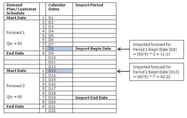
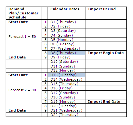
Following is an example of how this works:

Import Begin Date and End Date falls into two different forecasting periods.

Daily Distribution Method - Only in Import Demand Planning Forecasts

The imported forecasts are distributed and displayed on each day (workday for MRP spares) within the specified time period. The system calculates the daily forecast quantity by dividing the total imported forecast quantity by the number of days (workdays for MRP spares) which each forecast belongs to and insert each imported forecast on every day (working day for MRP spares) in the Date Range for the import. The system rounds up any fractional quantities and carries over any overages to the next day (next workday for MRP spares).

The following is an example of how this works.

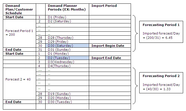
The system calculates the imported forecast as follows:

Forecast Date	Calculation	Distributed Forecast
D31 (Period 1)	6.45 ->rounded to 7, overage = 0.55	7
D30 (Period 1)	6.45 -0.55 = 5.9 -> rounded to 6, overage=0.1	6
D1 (Period 2)	1.33-0.1=1.23 -> rounded to 2, overage=0.77	2
D2 (Period 2)	1.33-0.77 =0.56 -> rounded to 1, overage=0.44	1
	And so on	.

Weekly Distribution Method

For the first week in the specified Date Range, the forecast is distributed and displayed on the Starting Date. (You can refer how starting and ending dates are calculated in the above section). For the following and each subsequent week, the imported forecast is distributed on Monday. The forecast quantity for each week is the sum of the forecast quantity for each day (working day for MRP spares) in the week. When it comes to MRP spares, if Monday is not a workday, then the forecast is added to the forecast of the previous week and displayed it on either the previous Monday or the Starting Date. If the forecast for the previous week does not exist, an error message will appear as well.

The following example uses data from the previous example to illustrate the weekly distribution method.

Distribution period falls into the Date Range where the Start Date is on D8 and End Date is on D19. Date Range consists of two different forecasting periods.

Using the above information, the system calculates the imported forecast as follows:
Imported Forecast = (Quantity/n)*N, where
Quantity = forecast quantity for the forecasting period
n = Number of days (work days for MRP spares for the forecasting period)
N = Number of days (working days for MRP spares) in import period within forecasting period.

Forecast Date	Calculation	Distributed Forecast
D8 (Start Date)	5.55*2-> 11.1 rounded to 12, overage = 0.9	12
D12 (Monday)	(8.88*6 -0.9) ->52.38 rounded to 53, overage 0.62	53
D19 (Monday)	8.88-0.62 ->8.26 rounded to 9, overage 0.74	9

Importing Demand Forecasts Overlapping the Master Schedule Time Fence Dates

If the Copy Forecast Inside Planning Time Fence setting is enabled (set to True) in the Import Demand Planning Forecasts assistant, and considering the import starting date if an exported forecast time period overlaps with the DTF date, then the forecast quantity in that exported forecast time period(which corresponds with the DTF date) is compared against the existing total forecast of MS Level 1 forecast 0 column for the same period up to the DTF date. This assess if there is a surplus forecast quantity to be imported from the exported forecast time period. If this surplus forecast quantity is less than the proportionated forecast quantity for the remaining days, then only the surplus forecast quantity is imported after the DTF date according to the chosen forecast distribution, otherwise the proportionated forecast quantity is imported.

A similar mechanism is there if the Copy Forecast Inside Planning Time Fence setting is not enabled (set to False) in the Import Demand Planning Forecasts assistant. Here the surplus forecast quantity is calculated based on the exported forecast period that corresponds with the PTF date, against the existing total forecast of MS Level 1 Forecast 0 column for the same period up to the PTF date.

Let’s consider a scenario where we’re importing a forecast for a part planned by MS, from today to one year ahead with Copy Forecast Inside Planning Time Fence setting not enabled (set to False).

Assume that the forecast periods are in months on the Exported Forecasts page. Let the PFT date of the part be on the 15th day (Day 15) in the next month and the corresponding exported forecast time period, from the 1st day (Day 1) to the end of the month (Day 31), has a forecast quantity of 3,100 on the Exported Forecasts page. There is already an existing forecast of 1,000 on Day 1, and 1,500 on Day 10, in Master Schedule Level 1 Forecast 0 column, and it will not be changed during the import job because we have set the Copy Forecast Inside Planning Time Fence to false. Hence, the forecast will be imported and distributed from Day 16.

During the import job, the proportionated quantity and the surplus are calculated as follows:

Proportionated quantity = 3,100/31×16 = 1,600 ;This is the exported forecast divided by the number of days in the period, multiplied by the remaining days from Day 16 to Day 31.
Surplus quantity = 3,100 − [1,000+1,500] = 600 ; This is the exported forecast minus the total forecast from Day 1 (the start date of the exported forecast period) up to Day 15th (the PTF date).

Since the surplus (600) is less than the proportionated quantity (1,600), only the surplus forecast quantity (600) will be imported and distributed according to the forecast distribution method. In another instance, if there is no surplus (i.e., 0), no forecast will be imported for that specific period or if the surplus forecast quantity is greater than the proportionated quantity, then the proportionated quantity will be imported. Similar mechanism is there for importing forecast from the exported time period that corresponds to the DTF date when the Copy Forecast Inside Planning Time Fence setting is enabled (set to True).

This approach ensures a smooth transition from planning and demand time fence dates and prevents from over-importing of forecast which may lead to excess supply.

Import Forecast by Customer Dimension

You can import forecasts from Demand Planner to Master Scheduling by Customer Dimension, using the Import Demand Planning Forecasts assistant and selecting the Import Type to Into Customer Dimension.

Forecasts are imported from Exported Forecasts By Dimension page, based on the customer dimension (Customer, Customer Stat Group, Market, Region, District or Country) that has been defined in the Demand Planner flow. It is mandatory that the same dimension is selected on the Forecast By field on the Master Schedule Level 1 Part page, otherwise, forecasts will not be imported.

The forecasts will be imported to the Forecast by Customer Dimension page. However, since these forecasts are automatically aggregated, they will also appear as total forecasts in the Master Schedule by Part page.

Dates, calculations, and distribution described earlier in this document are also applicable for import by Customer Dimension.

Import by Customer Dimension is available only from Demand Planner, not from Customer Schedules or from MRP Spare Parts.